Today in LabLulz, I’m going to walk through a recent preparation I did in my chemistry lab: increasing and measuring the concentration of hydrogen peroxide.
WARNING: This procedure involves heat and the end product is a powerful oxidizer. Don’t get burned and don’t get it on yourself – wear gloves, splash-resistant goggles, and an apron. I had a spill of ~15%, all over everything, including myself. It was okay, but only because I followed safety protocols. I didn’t have the apron though, and I had to get pantsless.
Hydrogen peroxide is an interesting substance; it’s formula is H2O2, meaning that it is composed of two hydrogen atoms bonded to two oxygen atoms.
It is a powerful oxidizer, decaying into water and free oxygen. This is because the bond between the two oxygen atoms, called the peroxide bond, is unstable. Some substances which contain the peroxide bond are even explosive, like triacetonetriperoxide. Because it’s an explosive precursor, and somewhat dangerous on its own, concentrated hydrogen peroxide can be difficult to come by. The weak 3% solution found in drugstores is all that is available to DIYers, hobbyists, and other scientists outside of the mainstream chemical supply chain.
Fortunately, it is relatively trivial to increase the concentration from 3% to around 30%. There are several tutorials on the subject at YouTube (TheChemLife; zhmapper, nerdalert226) so I’m going to focus on measuring the concentration of the end product, a procedure which the videos tend to treat very qualitatively. I hope this tutorial will be informative and useful, even outside of punklabs; the process is easily generalized and density is important in many fields, including medicine and winemaking.
The concentrating procedure is pretty simple: pour about 500 mL of the 3% solution into a beaker and heat it, forcing the excess water to evaporate until there is a tenth as much liquid left (peroxide boils at 150 C, compared to 100 C for water.) There are only a couple of tricky points: the liquid must NOT boil, only steam – if it starts boiling, the peroxide will decay. Bits of dust and dirt will also cause disintegration, so the equipment must be kept very clean and free from scratches.
Okay, so after a few hours, I have about 50 mL of liquid. I drop a bit into a solution of corn starch and potassium iodide, and the mixture turns black, a positive test for oxidizers. I add a squirt to some sulfuric acid and copper wire, and the metal wire begins bubbling and the solution begins to turn blue with copper sulfate*. This reaction is faster and more vigorous than when I try it with the 3% solution, so I’ve clearly succeeded in increasing the concentration, but to what level? To answer that question, I’m going to measure the density of the solution.

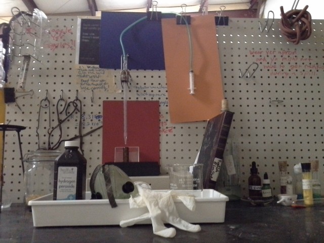
Figure 2. The Densitometry Setup. Note the safety equipment. Note also the lab notebook, which is essential. Other sights include a bit of iron oxalate, tongs, and a desiccator.
Here’s my setup. I don’t have a nice buret with a stopcock, so instead I have repurposed a graduated medical pipette (I picked up a huge box of these at the Scrap Exchange). This is controlled with a valve and a syringe plunger. It’s a little drippy and derpy, not great for dispensing a planned volume, but it works fine to measure the amount that has been dispensed, which is sufficient for our purposes. The milligram scale was lent to me by a friend after armed thugs stole my old one (thanks, B!) The brown glass vial is good for containing peroxide, since light speeds up its decomposition.**
Once the room and the beaker are at the same temperature (20 deg C), I draw about 8 mL of my peroxide up into the pipette, and start adding peroxide a bit at a time. By the time I had figured out the fluidics system, I’d added about 3.0 mL, so that’s where the data start. I then would squirt a bit of peroxide into the vial, note the volume and the mass, and repeat. I took 8 different measurements this way.
Then, after I put everything away and cleaned up, I sat down with a cup of coffee for a bit of data entry.

Figure 3. Data, in analog and digital form. This is a page from my lab notebook, and the spreadsheet in gnumeric (inset).
I usually store my data in spreadsheets, and my processing and analysis with Python. Once the spreadsheet file is ready, I get started and load up my data.
$ ipython –pylab
In [1]: import xlrd
In [2]: phial = xlrd.open_workbook('densityData.xls')
In [3]: data = phial.sheet_by_index(0)
In [4]: raw_volume = data.col_values(1)[5:]
In [5]: raw_mass = data.col_values(3)[5:]
Next, I take a quick peek at the data just to make sure that everything is as expected.
In [6]: plot(raw_volume, raw_mass, 'bo')
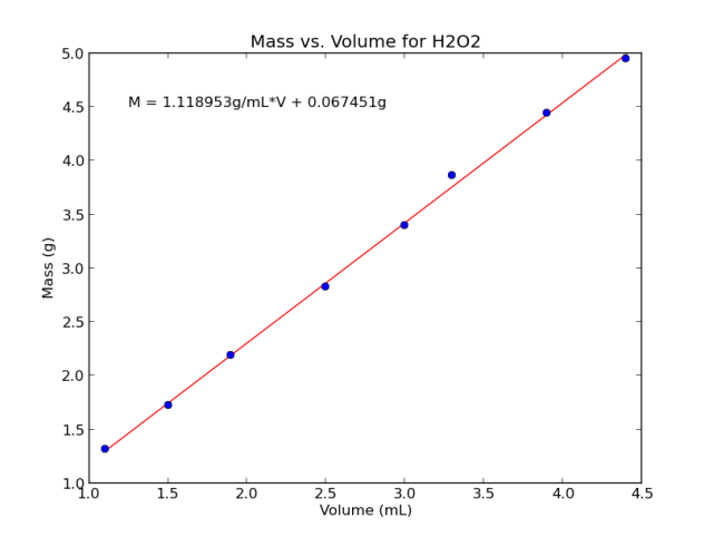
Looking good; the data are nice and linear, meaning that the slope (and therefor the density) is well defined. But this is the raw data, which include the mass of the bottle. I also didn’t start at zero on my pipette, just wrote down the volume the liquid was at when I took each mass measurement. It doesn’t matter too much, but strictly speaking, we want to compare just the mass of the liquid in the bottle to the volume of liquid drained from the pipette. Let’s go ahead and calculate that (it’s a lot like calculating temperature anomaly.)
In [12]: volume = array(raw_volume) - 3.0*ones_like(raw_volume)
In [12]: mass = array(raw_mass) -9.988*ones_like(raw_mass)
Much better. Now, to get some basic statistics on these data, let’s apply a linear regression.
In [13]: from scipy import stats
In [16]: (m, b, r, p, std) =stats.linregress(volume, mass)
In [17]: (m, b, r, r**2,  p, std)

Out[17]:
(1.1189534883720933,
0.067450581395348319,
0.99932418729044048,
0.99864883130369941,
7.7125664942037092e-10,
0.01680292147514929)
It’s mostly the slope, m = 1.12 g/mL, which we’re interested in.
In [16]: linFit = polyval([m,b], volume)
In [29]: plot(volume, linFit, 'r-')
In [30]: plot(volume, mass, 'bo')
In [31]: title('Mass vs. Volume for H2O2')
In [32]: xlabel('Volume (mL)')
In [33]: ylabel('Mass (g)')
In [36]: text(1.25, 4.5, 'M = %fg/mL*V + %fg'%(m,b))

Figure 4. The mass of peroxide is plotted as a function of its volume, and a linear regression applied.
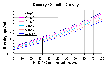
Now that we have the density, we can use this graph from H2O2.com. (It’s derived from Easton et al 1952. The paper actually reports on density measurements at 0, 10, 25, 50, and 96 degrees, so these are probably interpolated curves). We’ll draw a horizontal line at the measured density (~1.12 g/mL) until we hit the curve corresponding to the temperature (20C). Then we draw a vertical line and read off the concentration where it crosses the horizontal axis. Result? The concentration is about 32%. (Figure 5)
You may wonder why I went through so much trouble of taking multiple data points and calculating a trend line. If density is defined as mass per volume, then surely I can measure it in one go, by massing a single sample of known volume. Right? The problem is that any one such measurement might be a little wonky. Maybe one fewer drop than usual wiggled out, or a draft of air was pushing down a little on the scale. Look back at Figure 4; see the data point third from the end, visibly above the trend line? If I was only taking one measurement, I might get unlucky enough to get an outlier like that one. By using a linear regression, I can aggregate the data, and hopefully all those small outside factors will tend to cancel out.
Another reason is that the linear regression allows us to calculate uncertainty in the slope of the line, and therefor in the density. There are good online explanations of this, so I’m just going to churn through the equations.
In [26]: N = len(volume)
In [27]: unc = std *sqrt(N/(N*sum(volume**2)-sum(volume)**2))
In [28]: unc
Out[28]: 0.005463100999105781
We can thus report the density as 1.119 +/- 0.005 g/mL. If we wanted, we could use the uncertainty in the density to calculate the uncertainty in concentration the same way we calculated the concentration estimate: plot lines at 1.119 + 0.005 g/mL for the upper bound, and 1.119 – 0.005 g/mL for the lower bound and work backwards to get a confidence interval of concentrations. In our case though, the uncertainty is so small that it’s about the width of the original line not really worth propagating.
I feel comfortable just calling this 32% peroxide. Success!
* An easier, quicker test is to add peroxide to a catalyst that causes it to decay, but I didn’t have any manganese dioxide or horseradish on hand. Also, everyone loves copper sulfate.
** This is really a moot point, since I am keeping this sample in the fridge, and there is not even a lightbulb to philosophize about. But it’s also why you buy peroxide in opaque bottles.
~~~
Easton, M., Mitchell, A., & Wynne-Jones, W. (1952). The behaviour of mixtures of hydrogen peroxide and water. Part 1.?Determination of the densities of mixtures of hydrogen peroxide and water Transactions of the Faraday Society, 48 DOI: 10.1039/TF9524800796


Hey, so I tried it!
I heated 200ml of 6% hydrogen peroxide, keeping the temperature between 85 and 90 °C for 30-40 minutes. It made 40ml of concentrated peroxide.
Was too lazy to measure the new concentration, so I checked the difference between the peroxide in the bottle and the concentrated one, by testing it with the elephant toothpaste experiment (same proportions, only the concentration of the peroxide is different). It was clear that the reaction was more intense with the one I heated.
Conclusion : the method works!
– Jean-Boussole
Or you can purchase it in 35% concentration https://www.sklep.biomus.eu/pl/nadtlenek-wodoru-35-perhydrol/188-perhydrol-nadtlenek-wodoru-1l-5902409412222.html
Another method instead of boiling seems to be doing the opposite: freezing the solution and collecting the concentrated solution.
http://forums.welltrainedmind.com/topic/326082-chemistry-tip-concentrated-hydrogen-peroxide-cheaply/
Any comments on this? I haven’t bothered to try so no idea how well it works.
You could run the solution through a filter that contains carbon. A carbon block filter will remove the water, and allow the peroxide to exit the filter.
hm… I’d be concerned that the high surface area of the activated carbon would contain lots of nucleation sites for the peroxide to decompose on. Have you tried this before? I could give it a shot.
I get 30% or stronger H2O2 from “beauty supply” shops, like Sally’s, which supply hairdressers. This may be a good starting stock for higher concentrations. It’s actually more cost effective per unit of H2O2 than drug store 3%, and is also purer (else it would decay in storage.
For H2O2 at 30% or so, manganese dioxide can be obtained by opening a “dry cell” battery, putting the black goo in a filter paper/funnel and rinsing well with hot and cold water. The contaminant electrolytes in a cheap “heavy duty” cell (these are actually “low duty”; the label “heavy duty” was applied the 1960s, and battery technology has advanced in 50 years!), mostly ammonium chloride and nitrate, are generally innocuous, but not necessarily for *high* conc. H2O2! Alkaline cells share the same basic chemistry, but should be rinsed even more thoroughly. I use fresh batteries, because dead batteries will have more dissolved zinc, and I avoid metal ions near highly conc H2O2.
I was under the impression that, at least locally, they don’t sell peroxide to individuals; I had a vague memory of some bomb plot in which the makers had stolen peroxide from a beauty supply store, being unable to buy it. I could be wrong though; google is coming up with terrorists buying it, or in one case being a hairdresser themselves.
Since writing, I have indeed scavenged some batteries for their zinc, MnO2, and graphite rods. MnO2 is a mess to work with though, and the battery grade is mixed with graphite. I avoid it whenever I can so that I don’t have to clean.
Hydroponics stores and sometimes pool stores carry hydrogen peroxide at 30%.
I’ll keep an eye out, thanks! I’ve been meaning to drop by the pool store anyway for its halogen and pH compounds >.>
Hi, thanks for this! A lot of the DIY board folks are having problems getting >3% H2O2 and even this is getting hard to find due to stupid Govts ruining our fun.
Often the cheap stuff is contaminated with phosphoric acid, fumaric acid, corn starch and other garbage that ruins any possible etching of copper.
I did speculate that another way to make H2O2 is to use some sort of corona generator and bubble the ozone and NOx thus created through a filtering bath then triple distilled water creating both nitric acid or peroxide depending on the previous filtering.